Keyframe Animation

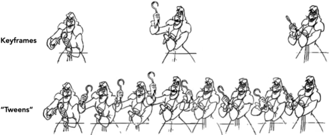
Animator creates keyframes.

Assistant creates in-between frames

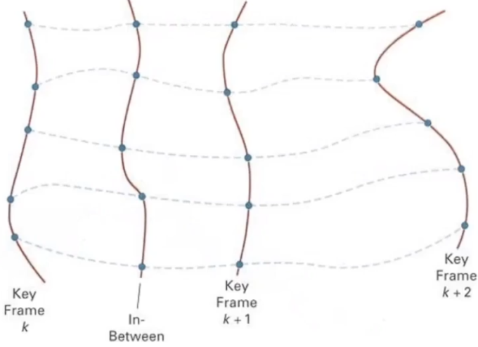
Keyframes Interpolation: Think of each frame as a vector of parameter values

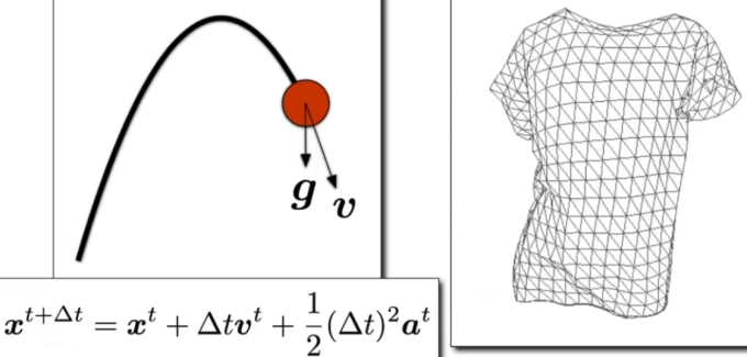
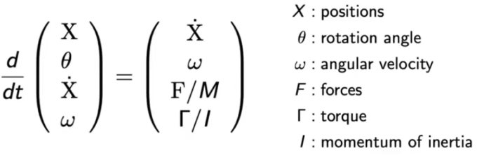
Physical Simulation

Newton's Law: $F(\text{Force})=m(\text{Mass})a(\text{Acceleration})$

Generate motion of objects using numerical simulation

Mass Spring System

Example of Modeling a Dynamic System

A Simple Spring

Idealized Spring:

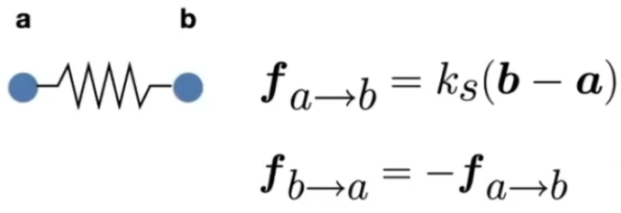
Force pulls points together.

Strength proportional to displacement (Hooke's Law)

$k_s$ is a spring coefficient: stiffness

Non-Zero Length Spring: Spring with non-zero rest length

$l$ is rest length

Problem: oscillates forever

If $\vec{x}$ is a vector for the position of a point of interest, we will use dot notation for velocity and acceleration: $\dot{x}=\vec{v}$, $\ddot{x}=\vec{a}$

Introducing Energy Loss: Simple motion damping $\vec{f}=-k_d\dot{b}$

• Behaves like viscous drag on motion
• Slows down motion in the direction of velocity
• $k_d$ is a damping coefficient

Problem: slows down all motion

Internal Damping for Spring: Damp only the internal, spring-driven motion $\Large\vec{f}_b=-k_d[\frac{\vec{b}-\vec{a}}{||\vec{b}-\vec{a}||}\cdot(\dot{b}-\dot{a})]\cdot\frac{\vec{b}-\vec{a}}{||\vec{b}-\vec{a}||}$

$\vec{f}_b$ : Damping force applied on b

$\frac{\vec{b}-\vec{a}}{||\vec{b}-\vec{a}||}(\dot{b}-\dot{a})$: Relative velocity projected to the direction from a to b (scalar)

$\dot{b}-\dot{a}$: Relative velocity of b, assuming a is static (vector)

$\frac{\vec{b}-\vec{a}}{||\vec{b}-\vec{a}||}$: Direction from a to b

• Viscous drag only on change in spring length

  Won't slow group motion for the spring system (e.g. global translation or rotation of the group)

• Note: This is only one specific type of damping

Structures from Springs

Behavior is determined by structure linkages

Particle Systems

Model dynamical systems as collections of large numbers of particles

Each particle's motion is defined by a set of physical (or non-physical) forces

Popular technique in graphics and games

• Easy to understand, implement
• Scalable: fewer particles for speed, more for higher complexity

Challenges

• May need many particles (e.g. fluids)
• May need acceleration structures (e.g. to find nearest particles for interactions)

Animation: For each frame in animation

• [If needed] Create new particles
• Calculate forces on each particle
• Update each particle's position and velocity
• [If needed] Remove dead particles
• Render particles

Forces

• Attraction and repulsion forces

  • Gravity, electromagnetism, ...
  • Springs, propulsion, ...

• Damping forces

  • Friction, air drag, viscosity, ...

• Collisions

  • Walls, containers, fixed objects, ...
  • Dynamic objects, character body parts, ...

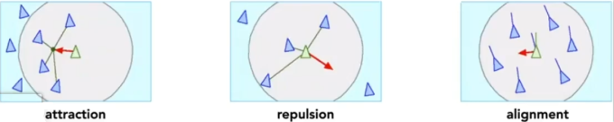
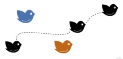
Simulated Flocking as an ODE

Model each bird as a particle. Subject to very simple forces:

• attraction to center of neighbors
• repulsion from individual neighbors
• alignment toward average trajectory of neighbors

Simulate evolution of large particle system numerically

Emergent complex behavior (also seen in fish, bees, ...)

Kinematics

Forward Kinematics

Articulated skeleton

• Topology (what's connected to what)
• Geometric relations from joints
• Tree structure (in absence of loops)

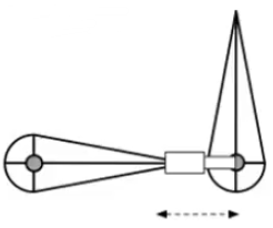
Joint types

• Pin (1D rotation)
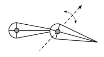
• Ball (2D rotation)
• Prismatic joint (translation)

Strengths:

• Direct control is convenient
• Implementation is straightforward

Weaknesses

• Animation may be inconsistent with physics
• Time consuming for artists

Inverse Kinematics

Animator provides position of end-effector, and computer must determine joint angles that satisfy constraints.

Direct inverse kinematics: for two-segment arm, can solve for parameters analytically.

Problem:

• Multiple solutions in configuration space
• Solutions may not always exist

Numerical solution to general N-link lK problem

• Choose an initial configuration
• Define an error metric (e.g. square of distance between goal and current position)
• Compute gradient of error as function of configuration
• Apply gradient descent (or Newton's method, or other optimization procedure)

Rigging

Rigging is a set of higher level controls on a character that allow more rapid & intuitive modification of pose, deformations, expression, etc.

Important:

• Like strings on a puppet
• Captures all meaningful character changes
• Varies from character to character

Blend Shapes

Instead of skeleton, interpolate directly between surfaces

E.g. , model a collection of facial expressions:

• Simplest scheme: take linear combination of vertex positions
• Spline used to control choice of weights over time

Motion Capture

Data-driven approach to creating animation sequences

• Record real-world performances (e.g. person executing an activity)
• Extract pose as a function of time from the data collected

Strengths

• Can capture large amounts of real data quickly
• Realism can be high

Weaknesses

• Complex and costly set-ups
• Captured animation may not meet artistic needs, requiring alterations

Particle Simulation

Single Particle Simulation

Assume motion of particle determined by a velocity vector field that is a function of position and time: $v(x,t)$

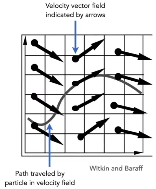
Computing position of particle over time requires solving a first-order ordinary differential equation(ODE):

Euler's Method

• Simple iterative method

• Commonly used

• Very inaccurate

• Most often goes unstable

• Errors: With numerical integration, errors accumulate. Euler integration is particularly bad.

• Instability: Inaccuracies increase as time step $\Delta t$ increases. Instability is a common, serious problem that can cause simulation to diverge.

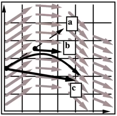
Combat Instability

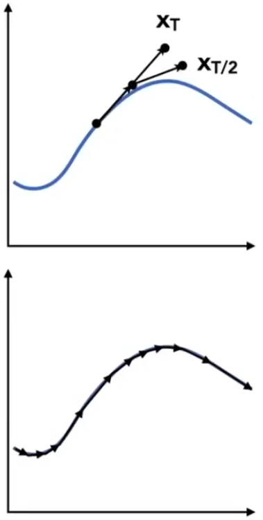
• Midpoint method / Modified Euler: Average velocities at start and endpoint

  Midpoint method:

  • Compute Euler step (a)
  • Compute derivative at midpoint of Euler step (b)
  • Update position using midpoint derivative (c)

  

  Modified Euler: Average velocity at start and end of step

• Adaptive step size: Compare one step and two half-steps, recursively, until error is acceptable

  • Technique for choosing step size based on error estimate
  • Very practical technique
  • But may need very small steps!

  Repeat until error is below threshold:

  • Compute $x_T$ an Euler step, size $T$
  • Compute $x_{T/2}$ two Euler steps, size $T/2$
  • Compute error $||x_T-x_{T/2}||$
  • If (error > threshold) reduce step size and try again

• Implicit methods: Use the velocity at the next time step (hard)

  • Informally called backward methods
  • Use derivatives in the future, for the current step
  • Solve nonlinear problem for $x^{t+\Delta t}$ and $\dot{x}^{t+\Delta t}$
  • Use root-finding algorithm, e.g. Newton's method
  • Offers much better stability

• Position-based / Verlet integration: Constrain positions and velocities of particles after time step

  • After modified Euler forward-step, constrain positions of particles to prevent divergent, unstable behavior
  • Use constrained positions to calculate velocity
  • Both of these ideas will dissipate energy, stabilize

  Pros / cons:

  • Fast and simple
  • Not physically based, dissipates energy (error)

Rigid Body Simulation

Simple case:

• Similar to simulating a particle
• Just consider a bit more properties

Fluid Simulation

• Assuming water is composed of small rigid-body spheres
• Assuming the water cannot be compressed (i.e. const. density)
• So, as long as the density changes somewhere, it should be "corrected" via changing the positions of particles
• You need to know the gradient of the density anywhere w.r.t. each particle's position

Large Collections

Two different views to simulating large collections of matters:

• Lagrangian Approach (质点法):

  Photographer follows the same bird through out its course.

• Eulerian Approach (网格法):

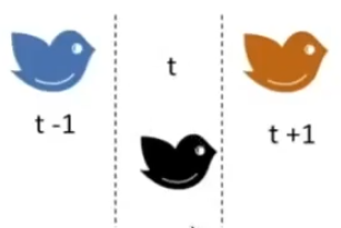
  The photographer is stationary and can take picture of all the birds passing through one frame only (say at time 't').

Material Point Method (MPM): Hybrid, combining Eulerian and Lagrangian views

• Lagrangian: consider particles carrying material properties
• Eulerian: use a grid to do numerical integration
• Interaction: particles transfer properties to the grid, grid performs update, then interpo-late back to particles